where the sum is to be taken over all paths
In a suboptimal search, which must be used in a real recognition system , there is no guarantee to find the global optimum as required by the Bayes decision rule. Therefore it is important to organise the search as efficiently as possible to minimise the number of search errors. Here, we will describe so-called time synchronous beam search which is the key component in many large vocabulary systems [Alleva et al. (1993), Fissore et al. (1993), Murveit et al. (1993), Soong & Huang (1991), Haeb-Umbach & Ney (1994), Valtech et al. (1994)].
Acoustic-phonetic modelling
is based on Hidden Markov models.
For an utterance to be recognised,
there is a huge number of possible state sequences, and all combinations
of state and time must be systematically considered.
In the so-called Viterbi or maximum approximation
[Bahl et al. (1983), Levinson et al. (1983)], the sum over all
paths is approximated by the path which has the maximum contribution
to the sum:

where the sum is to be taken over all paths ![]() that are
consistent with the word sequence
that are
consistent with the word sequence ![]() under consideration.
under consideration.

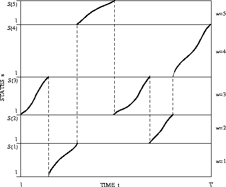
Figure 7.9: Example of a time alignment path
In the maximum approximation, the
search problem can be specified as follows.
We wish to assign each acoustic vector at time t
to a (state,word) index pair. This mapping
can be viewed as a
time alignment path, which is a sequence of (state,word)
index pairs (stretching notation):
![]()
An example of such a time alignment path in connected
word recognition is depicted in Figure 7.9.
The dynamic programming strategy to be presented
will allow us to compute the probabilities
![]()
in a left-to-right fashion over time t
and to carry out the optimisation
over the unknown word sequence at the same time.
Within the
framework of the maximum approximation, the dynamic programming
algorithm presents a closed-form solution for handling the
interdependence of non-linear time alignment , word boundary
detection and word identification in continuous speech
recognition.
Taking this strong interdependence into account has been
the basis for many different variants of dynamic programming
solutions to the problem
[Vintsyuk (1971), Sakoe (1979), Bridle et al. (1982), Ney (1984)].
The sequence of acoustic vectors extracted from the input speech
signal is processed strictly from left to right. The search
procedure works with a time-synchronous breadth-first strategy, i.e. all
hypotheses for word sequences are extended in parallel for each
incoming acoustic vector.
Originally, the dynamic programming strategy was designed for small vocabulary tasks like digit string recognition. To extend this algorithm towards large vocabulary tasks, there are two concepts that have to be added:

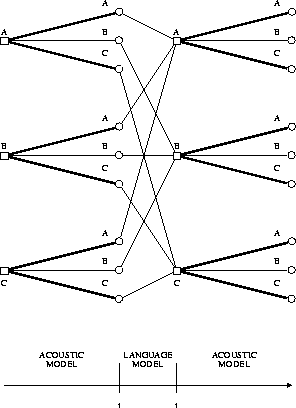
Figure 7.10: Bigram language model and search
Figure 7.10 illustrates how a bigram language model is incorporated into the search, where the vocabulary consists of the three words A,B,C. When starting up a new word w, all predecessor words v have to be considered along with their bigram probabilities p(w|v). Note that, since the bigram language model is a special case, the set of word sequences shown in Figure 7.2 can be compressed into a finite state network.
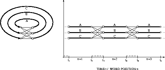
When using a lexicon tree to represent the pronunciation lexicon, we are faced with the problem that the identity of the word is known only when we have reached the end of the tree. The solution is to use a separate lexicon tree in search for each predecessor word [Haeb-Umbach & Ney (1994)] as illustrated in Figure 7.11.

Figure 7.11: Word recombination for a lexical tree
Fortunately, in the framework of beam search , the number of surviving predecessor words and thus the number of active trees is small, say 50 even for a 20000 word task with a perplexity of 200.
To prepare the ground for dynamic programming ,
we introduce two auxiliary quantities,
namely the score ![]() and the
back pointer
and the
back pointer ![]() :
:
Note that for both quantities, the index w is known only at the leaves of
the lexicon trees.
Both quantities are evaluated using
the dynamic programming recursion for ![]() :
:
![]()
where ![]() is the product of emission and transition
probability as given by the Hidden Markov model , and
is the product of emission and transition
probability as given by the Hidden Markov model , and
![]() is the optimum predecessor state for
the hypothesis (t,s;w) and predecessor word v.
The back pointers
is the optimum predecessor state for
the hypothesis (t,s;w) and predecessor word v.
The back pointers ![]() are propagated according
to the dynamic programming (DP) decision.
Unlike the predecessor word v,
the index w is well defined
only at the end of the lexical tree.
Using a suitable initialisation
for
are propagated according
to the dynamic programming (DP) decision.
Unlike the predecessor word v,
the index w is well defined
only at the end of the lexical tree.
Using a suitable initialisation
for ![]() , this equation includes optimisation
over the unknown word boundaries.
At word boundaries,
we have to find the best predecessor word
for each word.
To this purpose, we define:
, this equation includes optimisation
over the unknown word boundaries.
At word boundaries,
we have to find the best predecessor word
for each word.
To this purpose, we define:
![]()
To start words, we have
to pass on the score and the time index:
![]()
Note that here the right-hand side does not depend on
word index w since as said before the
identity of the spoken word is known only at the
end of a tree.
To measure the search effort there are a number of quantities that can be used: