Search: Word graphs

  The main idea of a word graphword graph word lattice is to generate word alternatives in regions of the speech signal, where ambiguity in the acoustic recognition is high. The advantage is that pure acoustic recognition is decoupled from the application of the language model and that a complex language model, for example a stochastic context free grammar,    can be applied in a subsequent postprocessing step. The number of word alternatives should be adapted to the level of ambiguity in acoustic recognition. The difficulty in efficiently constructing a good word graph is the following: the start time of a word depends in general on the preceding words. As a first approximation, we limit this dependence to the immediate predecessor word and obtain the so-called word pair approximation:

Given a word pair and its ending time, the word boundary  between the two words is independent of the further predecessor words.

This word pair approximation was originally introduced in [Schwartz & Austin (1991)] to efficiently calculate multiple or n-best sentences. The word graph can be expected to be more efficient than the n-best approach. In the word graph approach, word hypotheses need to be generated only locally whereas in n-best methods each local alternative requires a whole sentence to be added to the n-best list. To give an oversimplified example, as shown in Figure 7.12, suppose we have 7 spoken words and 2 word hypotheses for each word position. The n-best method then requires =128 sentence hypotheses, whereas the word graph approach produces a graph of only word arcs.

 
Figure 7.12: Simplified example of a word graph 

There have been a number of attempts at using two explicit levels in search: the first level produces a short list of either single word or sentence hypotheses, and at the second level, the final decision is taken using a complex language model [Sakoe (1979), Schwartz & Austin (1991), Soong & Huang (1991), Ney & Aubert (1994), Fissore et al. (1993), Oerder & Ney (1993), Woodland et al. (1995)]. In the following, we will describe a method for word graph generation based on word pair approximation. This method has been used successfully in two independent systems for 20000-word recognition [Ney & Aubert (1994), Woodland et al. (1995)]. The fundamental problem of word graph construction is:

• Given a word w and ending time t, how can we find a limited number of ``most likely'' predecessor words?
• This task is difficult since the start time of word w may very well depend on the predecessor word under consideration, which results in an interdependence of start times and predecessor words.

The basic idea is to isolate the probability contributions of a particular word hypothesis with respect to both the language model and the acoustic model. This decomposition can be visualised as follows:

The set of likely word sequences is represented by a word graph, in which each arc represents a word hypothesis. Each word sequence contained in the word graph should be close (in terms of scoring) to the single best sentence produced by the one-pass algorithm. We prefer the term ``word graph'' to ``word lattice''  to indicate that when combining word hypotheses, we do not allow overlaps or gaps along the time axis. When using an m-gram language model   , we can recombine word sequence hypotheses at the phrase level if they do not differ in their final (m-1) words. Therefore it is sufficient to distinguish partial word sequence hypotheses only by their final words . To describe the word graph construction algorithm, we introduce the following definitions:

• probability that word w produces the acoustic vectors .
• : (joint) probability of generating the acoustic vectors and a word sequence with the final words :
  
  where, as expressed by the notation, the final portion of the word sequence is not subjected to the maximisation operation.

 
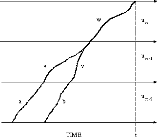
Figure 7.13: Word pair approximation 

Using the above definition, we can write the dynamic programming  equation at the word level:

 

Here we have used the function to denote the word boundary  between and for the word sequence with final portion and ending time t. To achieve a better pruning effect, a bigram  language model is included. The word boundary  itself is defined by a maximisation operation:

So far this has been just a notational scheme for the word boundary  function . The crucial assumption now is that the dependence of the word boundary can be confined to the final word pair . The justification is that the other words have virtually no effect on the position of the word boundary  in the word pair [Schwartz & Austin (1991)]. This so-called word pair approximation is illustrated in Figure 7.13. From this figure, it is obvious that the assumption of the word pair approximation is satisfied the better the longer the predecessor word is: all time alignment  paths then are recombined before they reach the final state of the predecessor word. We express this word pair approximation by the equation:

As long as only a bigram  language model is used, the word pair approximation is still exact (within the beam search  approximation).

To compute the word boundary  function , we have to distinguish the hypotheses in dynamic programming  according to the predecessor word, and we therefore use the predecessor conditioned algorithm. We add two equations, namely one for calculating the word boundary  function and one for calculating the word score . The word boundaries  are obtained using the back pointers at the word ends:

For each predecessor word v along with word boundary  , the word scores are recovered using the equation:

where we obtain H(w;t) according to its definition:

The details of the algorithm are summarised in Table 7.6. The operations are organised in two levels: the acoustic level and the word pair level. At the end of the utterance, the word graph is constructed by backtracking through the bookkeeping lists.

 

trace back: single best sentence and word graph

 

What has to be added to the single-best one-pass strategy is bookkeeping at the word level: rather than just the best surviving hypothesis, the algorithm has to memorise all the word sequence hypotheses that are recombined into just one hypothesis to start up the next lexical tree (or word models ). In the single-best method, only the surviving hypothesis has to be kept track of. To reduce the memory cost, a method for removing obsolete hypotheses must be included along with list organisations and dynamic construction of the search space [Ney et al. (1992)]. Given the word graph and the language model, the final search can be carried out at the word level using a left-to-right dynamic programming  algorithm as shown in Table 7.7. The cost of this search through the word graph depends on the complexity of the language model. For a trigram  model, it is typically less than 1% of the effort for constructing the word graph.

An example of a word graph for a three-word vocabulary  A,B,C including silence at the sentence beginning and end is shown in Figure 7.14 on page .

 
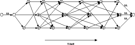
Figure 7.14: Example of a word graph 

The arcs stand for word hypotheses, whereas the circles along with the word name denote the word end. In this figure, the word pair approximation is reflected by the fact that the nodes  are labelled with the identity of the incoming words and thus the dependence on the predecessor word can be taken into account. In reality, the word graph is more complicated because we have to allow for optional silence between the words.

When we try to measure the efficiency of a word graph, it is evident that there are two important quantities to be considered, namely the size of the word graph and its quality in terms of errors. Obviously, the two quantities are dependent on each other. We try to specify how they could be measured:

• size of the word graph: We can measure the number of arcs and nodes  and normalise them with respect to the number of actually spoken words to account for different sentence lengths.
• errors of the word graph: What we want to know is how well is the actually spoken word sequence represented by the word graph? An error is encountered when there is no path through the word graph for the spoken word sequence. Such an error can be related to a word substitution , a word deletion  or a word insertion . To calculate the exact number of word errors, the so-called Levenshtein distance is extended to compute the best path for the spoken word sequence through the word graph, where we allow for word substitutions , word deletions  and word insertions.