In linear interpolation, a
weighted average between the relative frequencies ![]() and the
general distribution
and the
general distribution ![]() is computed:
is computed:
![]()
In leaving-one-out , we have to renormalise by the following substitution:
![]()
The leaving-one-out likelihood function is:
![]()
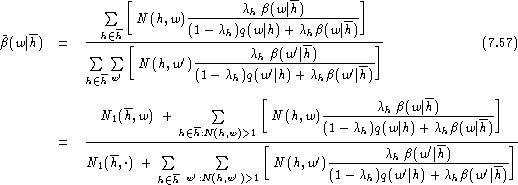
Taking the partial derivatives and doing some term rearrangements using q(w|h)=0 for N(h,w)=1, we obtain the iteration formulae [Ney et al. (1994)]:
Similarly, we have for the ![]() :
:

Again, the dominating effect of the singletons is evident.
For the special choice ![]() if N(h,w)>0, we have
linear discounting again and recover the corresponding equations.
if N(h,w)>0, we have
linear discounting again and recover the corresponding equations.
The model of linear interpolation considered so far is special
because it involves only two types of histories, namely h and ![]() .
In general, we may have several generalised histories
.
In general, we may have several generalised histories ![]() for i=1,2,....
For this general case of linear interpolation, the so-called EM algorithm provides
an efficient iterative procedure for estimating the unknown parameters
[Baum (1972), Dempster et al. (1977), Jelinek & Mercer (1980)]. To consider the details of the EM
algorithm , we have to specify the full interpolation model:
for i=1,2,....
For this general case of linear interpolation, the so-called EM algorithm provides
an efficient iterative procedure for estimating the unknown parameters
[Baum (1972), Dempster et al. (1977), Jelinek & Mercer (1980)]. To consider the details of the EM
algorithm , we have to specify the full interpolation model:

For the interpolation to work, the interpolation parameter ![]() must explicitly depend on the index i of the generalised history.
The framework of the EM algorithm is based on the so-called
must explicitly depend on the index i of the generalised history.
The framework of the EM algorithm is based on the so-called ![]() function, where
function, where ![]() is the new estimate obtained from
the previous estimate
is the new estimate obtained from
the previous estimate ![]() [Baum (1972), Dempster et al. (1977)].
The parameter
[Baum (1972), Dempster et al. (1977)].
The parameter ![]() stands for the whole
set of parameters to be estimated.
The
stands for the whole
set of parameters to be estimated.
The ![]() function is an extension of
the usual log-likelihood function and is for our model:
function is an extension of
the usual log-likelihood function and is for our model:

Taking the partial derivatives with respect to ![]() and observing the normalisation constraint,
we obtain the equation:
and observing the normalisation constraint,
we obtain the equation:
![]()
In this form, the interpolation parameters ![]() depend on the history h the number of which can be large.
Therefore, some sort of tying might often be useful [Jelinek & Mercer (1980)].
depend on the history h the number of which can be large.
Therefore, some sort of tying might often be useful [Jelinek & Mercer (1980)].
Taking the partial derivatives with respect to
![]() and observing the normalisation constraint,
we obtain the equation:
and observing the normalisation constraint,
we obtain the equation:
