The model of linear discounting in conjunction with backing-off [Katz (1987), Jelinek (1991)] has the advantage that it results in relatively simple formulae. The model is:

Here we have two types of parameters to be estimated:
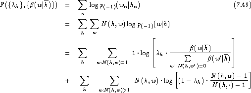
The unknown parameters are estimated by maximum likelihood in combination with leaving-one-out . We obtain the log-likelihood function:

where ![]() denotes the probability
distribution for leaving out the event (h,w) from the
training data .
denotes the probability
distribution for leaving out the event (h,w) from the
training data .
By doing some elementary manipulations, we can decompose the log-likelihood
function into two parts, one of which depends only on ![]() and the
other depends only on
and the
other depends only on ![]() :
:
![]()
The ![]() dependent part is:
dependent part is:

Taking the partial derivatives with respect to ![]() and equating them to zero, we obtain
the closed-form solution:
and equating them to zero, we obtain
the closed-form solution:
![]()
The same value is obtained when we compute the probability mass of unseen
words in the training data for a given history h:
![]()
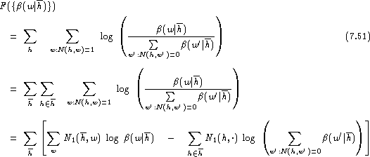
To estimate the backing-off distribution ![]() ,
we rearrange the sums:
,
we rearrange the sums:

where ![]() is the number of singletons (h,w) for a given history h,
i.e. the number of words following h exactly once, and where
is the number of singletons (h,w) for a given history h,
i.e. the number of words following h exactly once, and where ![]() is defined as:
is defined as:
![]()
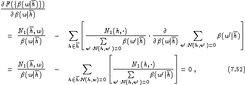
Taking the derivative, we have:

where we have taken into account that there are only contributions
from those histories h which appear in the sum over w'.
We do not know a closed-form solution for ![]() .
By extending the sum over all histories h [Kneser & Ney (1995)],
we obtain the approximation:
.
By extending the sum over all histories h [Kneser & Ney (1995)],
we obtain the approximation:
![]()
For convenience, we have chosen
the normalisation ![]() .
This type of backing-off distribution will be referred to as
singleton distribution.
.
This type of backing-off distribution will be referred to as
singleton distribution.